
Continuous Process Manufacturing Is Different
August 11, 2026
Lean in Continuous Manufacturing Insights
Michael L. George – Lucentryx Chairman of the Board
Mark Price – Lucentryx President
Critical Insights for Lean Implementation in Continuous Process Manufacturing
Why is Lean Different in Process Industries?
Globally, lean has achieved widespread adoption in the world of discrete manufacturing. In our experience continuous process manufacturers are still scratching the surface.
In continuous process manufacturing (such as metals, fiberglass, chemicals, food / beverage, pharmaceuticals, paper and packaging, adhesive application), implementing Lean manufacturing creates several challenges absent in discrete manufacturing, the birthplace of Lean (and notoriously through the Toyota Production System1). The continuous process manufacturing industry possesses two major differences:
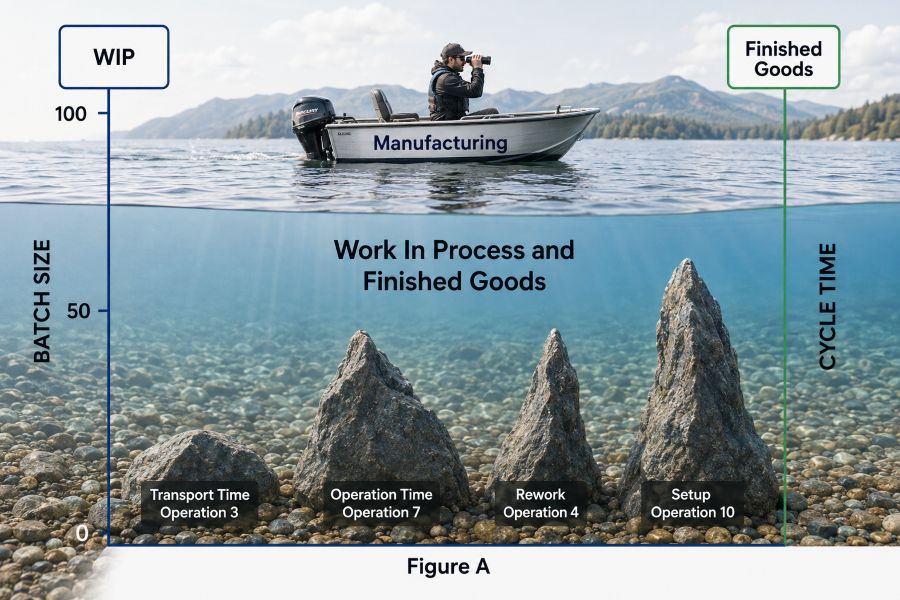
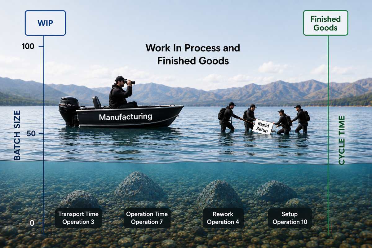
Discrete manufacturing has more Work-in-Process (WIP) inventory in buffers and batched queues. As illustrated in Figure 1, the water line represents the inventory that covers the manufacturing process deficiencies identified as rocks on the sea floor. The traditional Lean or Toyota Production System approach to improving manufacturing speed (cycle time), in discrete applications, targets “lowering the water level” exposing manufacturing process waste also known as T.I.M.W.O.O.D. As WIP reduces, forms of waste and non-value-added time are illuminated and easily seen. Process industries often have little or no WIP. The concept of accelerating manufacturing cycle time through lowering the water level does not easily translate because there is typically minimal WIP or water level present in continuous process environments. So, another cycle time reduction lever must be pulled to improve manufacturing speed.
Process industries are typically characterized by high fixed capital-intensive equipment, concentrated in a small number of large workstations. The production equipment is often physically large, relatively fixed in nature and often referred to as “monuments” across the industrial base. In most discrete manufacturing operations, the capital investment is typically smaller, spread across many workstations and flexible for relocation. As a result, continuous process manufacturing operations are less flexible to change than discrete manufacturing operations. For example, the smaller more flexible equipment found in discrete lends well to the creation of cellular manufacturing. This typically cannot be achieved to the same level of perfection with “capital monuments” found in continuous process manufacturing.
These problems were mitigated in the original formulation of the Toyota Production System by Heijunka which maintains the leveled sequencing of variants (complexity of different products). This method is also known as “Production Smoothing2” in the discrete manufacturing of the Toyota Production System. Toyota initially only produced 2 types of different cars on a single production line. The workstations thus only produced two different part numbers which were stored in local Kanban boxes. When the inventory was depleted to the minimum level, the workstation would changeover tooling to replenish inventory of 1 of the 2 part numbers. Setup time was reduced below 10 minutes using the Four Step Rapid Setup method7. When Toyota increased from 2 to 4 part numbers per workstation, the increasing Complexity was catastrophic according to “Toyota Troubles: Fighting the Demons of Complexity9”. This is now mitigated in discrete manufacturing by the AI LLM Complexity reduction process of Lucentryx.
This process has become more challenging as the number of end-item product variants has proliferated. From 1995-2005, our engagements with clients such as Colgate-Palmolive, Noble, Teledyne Wah Chang, Olin Brass, Hill’s Pet Nutrition, Owens-Corning, Alcan and many others applied an analytical, as opposed to trial and error, method of responding to the challenges described above in continuous process Lean applications.
The primary goals of Lean are to improve speed by reducing factory lead time and to improve the costs of waste by reducing inventory and delivering Just-In-Time3. In addition to the benefits of significantly improved customer service level through faster lead time, inventory reductions in the range of 70% dramatically reduce manufacturing overhead waste and downstream distribution and warehousing costs and immediate improvement to the spread between Return on Invested Capital (ROIC) and the Weighted Average Cost of Capital (WACC)4. Further, faster cycle times enhance the power of Six Sigma quality tools such as Design of Experiments by providing experiential data more rapidly. We place these challenges in context by first discussing the foundations of Lean.
Foundations of Lean
The mathematical foundation for Lean is Little’s Law4,6.

Little’s Law shows how lead time is related to the number of things in process (TIP or WIP) and the completion rate of the process or exit rate. There are clearly two ways to reduce lead time of any manufacturing or transactional service process:
- Reducing the numerator (WIP and FG inventory) or
- Increasing the denominator (production capacity / throughput)
Reducing inventory typically only requires investment in intellectual capital (Lean methods and application of the “creativity before capital” credo) whereas large increases in capacity frequently require investment in people and financial capital, with a negative impact on ROIC4. It is common to experience throughput increases as waste is eliminated via Lean methods as value-added processing time can be improved and waster elimination achieved simultaneously. The potential pitfall (regardless of the path for creating more production capacity) is the creation of excess capacity beyond market demand which can lead to overproduction – the most deadly of the Seven Deadly Wastes of Lean. In continuous process industries, the number of units of WIP and Finished Goods is primarily driven by the length of the run of each different product.
Unlike discrete manufacturing, WIP in continuous process industries is usually small since the product often flows through the process rather quickly and rarely waits while in process.
However, Finished Goods is typically large, since the time to cycle through ALL different products (defined as Workstation Turnover Time6) can be long and inventories must supply average demand during this cycle.
This is especially true when there is large product variety. Traditional Lean refers to long Workstation Turnover Time by referring to it as “unsmoothed production”. It will be shown below that the number of units of WIP and Finished Goods, and hence the cycle time is primarily driven by length of the run. We will also show that the length of the run is related to the duration of the setup time, quality, downtime and other process characteristics. We conclude that WIP, Finished Goods and lead time can be minimized in continuous process manufacturing industries when the minimum safe run length (or batch size) is launched and throughput increased. This minimum safe run length will be consistent with existing customer demand, setup times and other process characteristics. One of the most important formulas which defines this minimum run length or batch size is derived below.
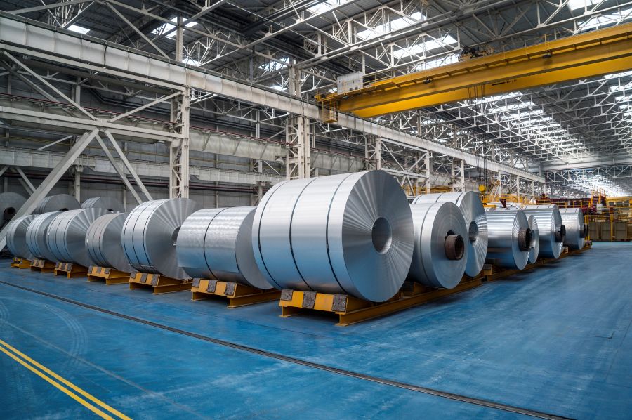
Cold Rolled Steel Continuous Manufacturing
“Trial and Error” versus Analytical Run Length Calculations
The assertion of Lean is that companies are currently launching batch sizes that are larger than required. These large batches create excess WIP and Finished Goods inventory which extend cycle time and mask waste. This waste may take the form of setup time, downtime, non-standard work, defects (rework), scrap, transportation & conveyance and other process deficiencies which cause large inventories, excessive overhead and quality cost. Application of the standard Lean prescription would recommend gradually reducing the batch size (by removing Kanban cards) until one of the workstations can no longer keep up with demand and the takt-time bar chart is unbalanced. This is generally caused because a workstation spends too large a percentage of time in setup (due to ever smaller batches and hence more setup) or in maintenance/repair, generates too much rework or scrap and too little time actually producing product. This is often referred to as “hitting the rocks” in Figure 2 below.
The failure to meet desired output can be mitigated in discrete manufacturing by placing temporary excess WIP buffer stocks and queues at the workstation under investigation. This is generally not possible in continuous process industries because it is a “straight through” process. In discrete manufacturing, each item of WIP is used in many different finished goods items. In process industries each run typically produces a unique end item, leading to larger excess inventory and slow Finished Goods turns. Thus the “trial and error” approach to finding the minimum safe run length and prioritizing improvements is not as feasible in continuous process industries.
Excess inventory is analogous to the water covering the rocks of waste, which are disclosed by lowering the “water level” (batch size). “Hitting the rocks” is the signal to apply the Four Step Rapid Setup Method (SMED), Total Preventive Maintenance (TPM), Operational Equipment Effectiveness (OEE) or other appropriate Lean methods and tools to that workstation. In this case attaching Operation 10 first in Figure 1.
Analytical Run Length Sizing Does NOT Equal EOQ!
Analytical run length (ARL) sizing uses data on setup time, demand, downtime and other real manufacturing process characteristics. ARL also considers the effect of the confluence of other products that share equipment to compute the safe minimum run length, (i.e., at the water level of the Rock) so that improvements can be applied before the process hits a rock. This approach differs distinctly from simple Economic Order Quantity (EOQ) batch sizing. EOQ computes run sizes for each part number independently. The EOQ calculation does not recognize process capability nor does it calculate the effect of a confluence of parts across a particular workstation. Rather the batch size calculated by EOQ remains constant whether 1 part or 1000 parts run across a given workstation. Our analysis has shown that EOQ frequently calculates batch sizes much larger than the minimum dictated by the characteristics of the process. We can illustrate analytical batch sizing to determine the minimum safe batch size (run length) by a simple example which can be easily generalized as in Figure 2 below.
Let us assume an extrusion machine produces only two different products, A and B. Let us assume that it takes two hours to perform a setup between a run of A and a run of B (and vice versa), and that the mill or extrusion line can operate at 100 feet per minute (6000 feet per hour) after setup is completed. Let us assume that the average demand for both product A and B is 2700 feet per hour. The factory is currently meeting demand, and is using a run length of 132,000 feet. What is the minimum safe run length that will minimize inventory and lead time and still meet the customer demand?
Essentially, the extrusion machine sets up for 2 hours, then runs 132,000 feet of product A which takes it 132,000/6000 or 22 hours, then uses 2 hours of setup time to prepare for product B. This cycle is shown below in the Inflexibility Diagram below:
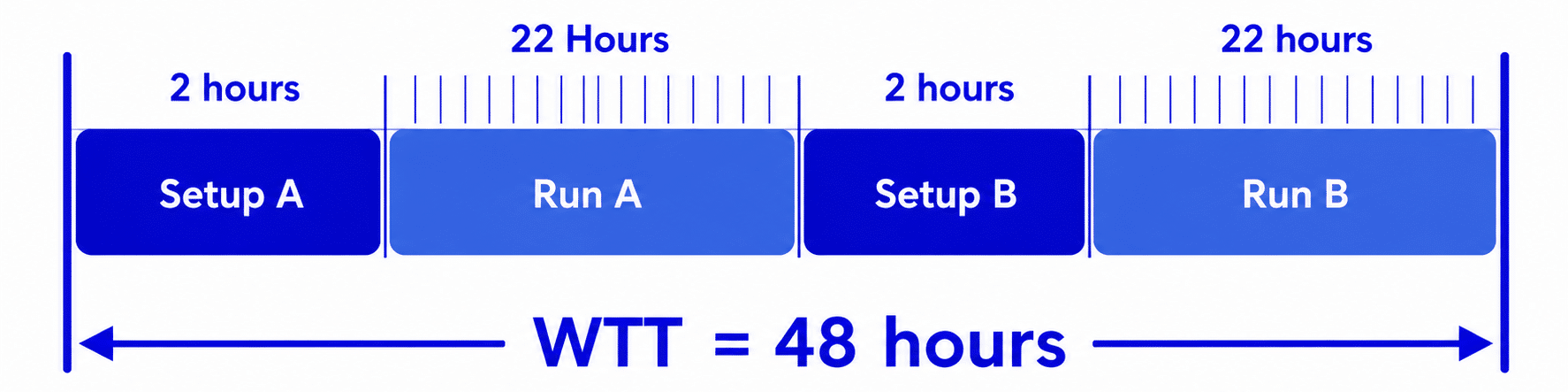
You will notice that the extrusion machine completes a cycle through all runs every 48 hours. This is known as the current total Workstation Turnover Time (WTT). This run length is clearly large enough because the company is meeting all demand, but it has lots of finished goods on hand. In fact, every 48 hours it produces 132,000 feet of each product, which amounts to:

The same is true for Product B. This is actually more than the 2,700 feet per hour demanded by customers. Overproduction is one of the Seven Deadly Wastes of Lean. By how much is the run length too large? Where is the rock? Is this causing a big cost and delivery problem? Should we worry about it?
We can calculate the minimum safe run length (i.e., location of the top rock under the water) by letting the run length be a variable for which we solve. Let’s build the Inflexibility Diagram again, using the run length in feet as a variable R. The first element of the Workstation Turnover Time is the setup time which is still 2 hours. The next element is the run time. We are running a length or R feet and have not yet determined the magnitude of R. At the rate of 6000 feet per hour, we are running each product for R/6000 hours after setup is complete, as is shown below.
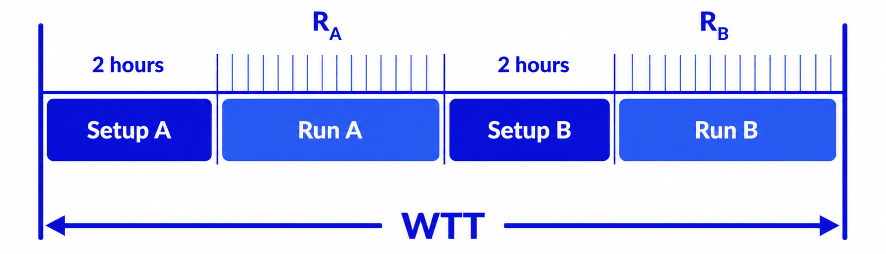
Setting Run Length As A Variable
We can now use the formula we developed above

And SU = setup time for Runi and P = processing time per unit for Runi. Solving for R, we have:
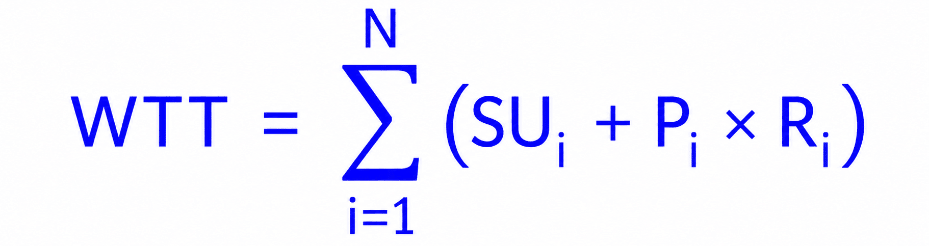
And SU = setup time for Runi and P = processing time per unit for Runi. Solving for R, we have:
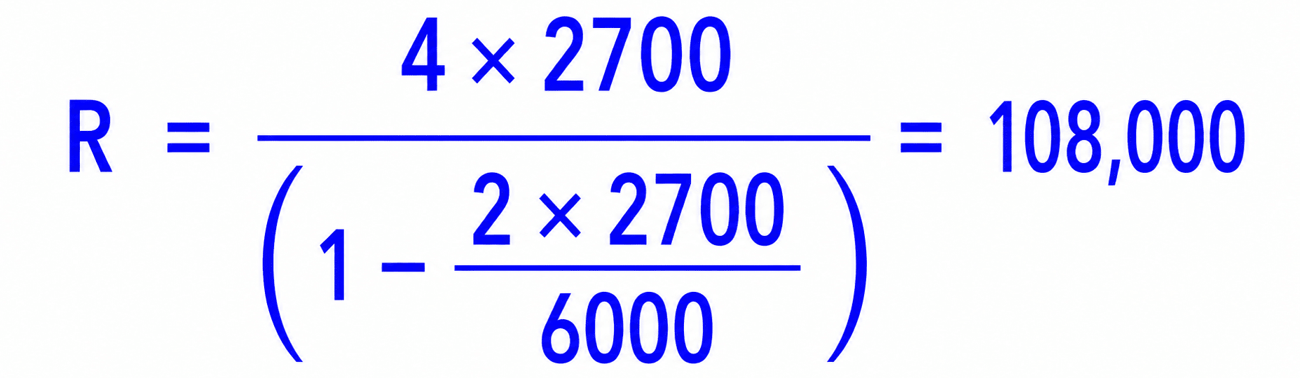
This proves we can immediately reduce our run length from 132,000 to 108,000 to the level of the rock (see Figure B below) and still meet demand. In the process, we will reduce finished goods inventory and lead time by 19%, also making the process more flexible to changes in customer demand.
Further, if the extrusion workstation is the one that requires the longest run lengths, then it is creating the greatest amount of inventory and the longest lead time delay…and is referred to as the leading Time Trap. The average delay that a workstation injects into a process is approximately half the Workstation Turnover Time. The sum of these delays down the critical path is the total lead time of the process for that product. Of greater importance in a continuous process industry is the time it takes to cycle through all the products and return to the starting point which creates the need for huge finished goods inventories as described above.
Prioritizing Process Improvements
Given the data in the figure above, we would focus the highest priority of effort on applying the Four Step Rapid Setup8 method to the extruder (Operation 10). Cutting its setup time in half (50%) will allow us to reduce the run length by 50% and delay time by half and still meet demand…but with half the inventory and lead time! In fact, setup times have been reduced from 4 hours to less than 10 minutes using this method.
It should be pointed out that setup time is not the only cause of long run lengths. Scrap, rework, machine downtime, and product proliferation (complexity) are often even larger drivers of long lead time. The impact of these factors on lead time is derived in US Patents (application note for the interested reader). The method can be easily generalized to show the impact of scrap, rework, machine and human downtime, and other factors. In Table 1 below, we present real results applying the minimum safe batch size and lean principles approached in continuous process manufacturing environments for specific workstations.
|
Bottleneck Cause (Process Deficiency) |
Process Change |
Resulting Lead Time Improvement |
Resulting Inventory Decrease |
|---|---|---|---|
|
Scrap Rate |
Reduced from 10% to 0% |
40% |
53% |
|
Long Setup Time |
Reduced from 8 to 4 hours |
50% |
50% |
|
Downtime / OEE |
Reduced from 10% to 0% |
33% |
33% |
|
Process Time / Unit |
10% reduction |
20% |
20% |
|
Process Flow Time |
10% reduction |
10% |
10% |
What percent of workstations destroy 80% of supply chain velocity? Only 20%!
The data table above can be turned to view it another way. For example, if you reduce setup time from 8 to 4 hours you will reduce inventory by 50%. Another cause of excess inventory is variation in demand mix. Some variation is just part of normal business and must be buffered out by finished goods inventory. However, if you can cut the run length in half, you cut the time to cycle through all the products in half and achieve a “leaner” production schedule. This will allow you to cut the variation buffer in half as well. Seasonal variation in total demand does require some “build ahead” inventory. Again, with faster cycle time, the “build ahead” can be focused on a few high-volume products.
Leveraging Improvement Efforts
We can also turn the logic around — if you have process deficiencies, there is an opportunity to accelerate the velocity of the supply chain. In real factories, it turns out that only about 20% of the workstations are responsible for destroying 80% of the velocity thus, improving only 20% of the workstations results in a five-fold increase in supply chain velocity. Managers are attracted by this leverage offered by continuous improvement. The insight that a 10% scrap rate can create a 53% increase in inventory and slow down the supply chain velocity by 38% is extremely compelling. Since many overhead costs, such as Distribution Centers, are quantized, significant cycle time and inventory reductions are required to remove these costs.
The Supply Chain Link
In practice, optimization of WTT drives Oder Frequency (or Cycle Time Interval – CTI) utilized for Enterpise Resource Planning (ERP) or Materials Resource Planning Systems (MRP). Lean application of WTT enables more resilient supply chains for ordering raw materials, components, packaging and planning of warehousing and other transportation and logistics requirements. WTT and thus CTI drives batch size or order quantities using actual manufacturing process data parameters which directly impact procurement of upstream requirements.
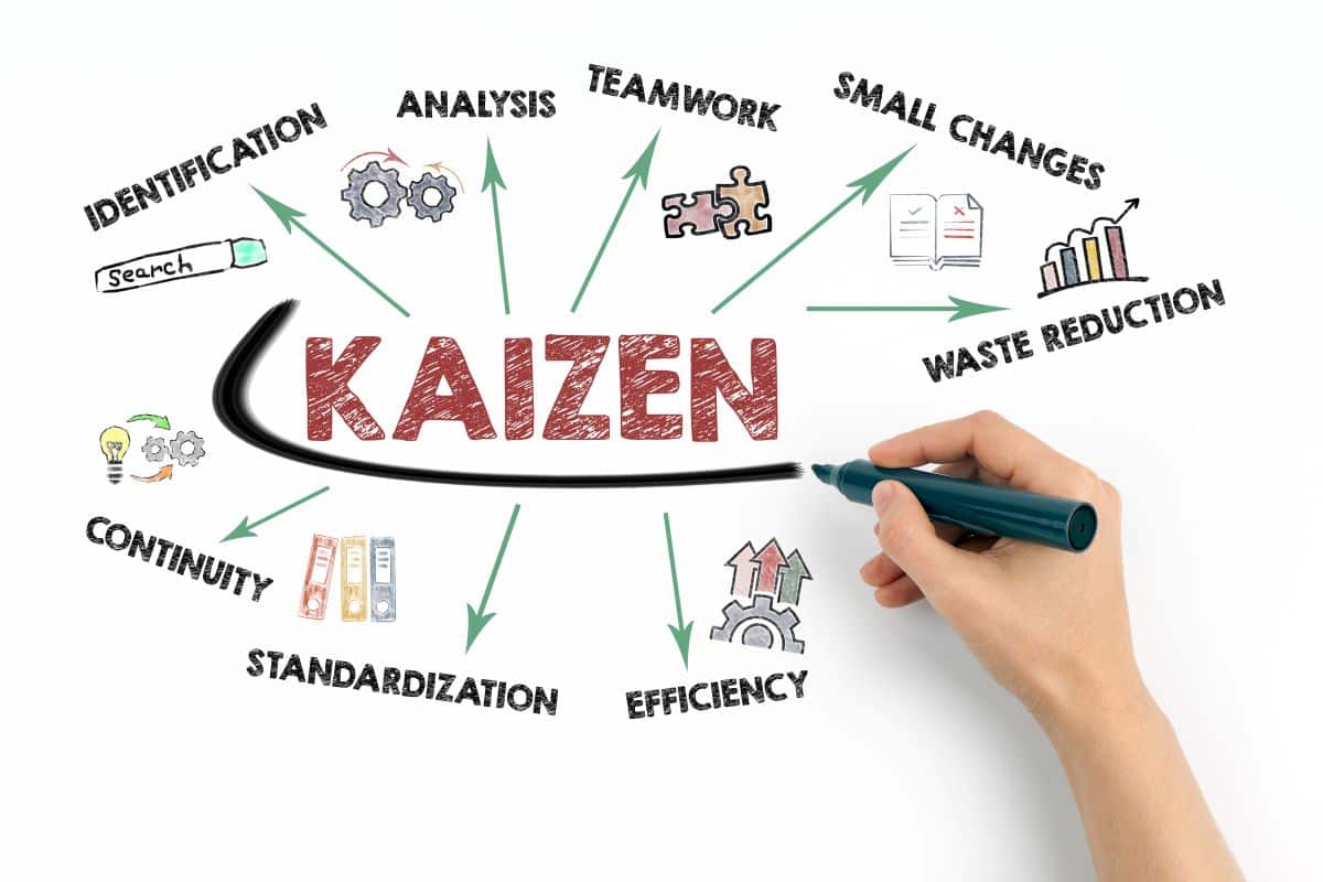
Improving the Process using Kaizen events:
“Drive-By” Kaizen, or Kaizen Prioritized by Analytics?
Lean is about continuous improvement with the goal of attaining >20% Process Cycle Efficiency6. In discrete manufacturing, the power of the Kaizen event has been responsible for shop floor excellence, team work and tactical operational excellence. In a Kaizen event, operators from the suspect process or workstation work with a Lean Master for 3-5 days to quickly apply the Four Step Rapid Setup method or other Lean methods. This action-oriented process makes use of the data and deep tacit process knowledge of process owners and participants in an implementation-focused workshop. The alternative approach is to just use intuition, and do scores of Kaizen events per year until nearly every suspect workstation has been “Kaizened” with slow average reductions in batch size, with buffers and quick reaction to line stoppage.
The problem with this approach is that “Kaizening” a workstation that is not injecting much time
delay has no benefit in the plant wide cycle time reduction process and often results in “islands of excellence” with no overall value stream benefit. These are the so-called “Drive by” kaizen events which may be an excellent application of Lean tools, but unfortunately to the wrong workstation and with no thought about the entirety of the value stream. While Kaizen events generate a lot of shop floor enthusiasm, they must provide lasting financial benefit through lower costs, faster lead time and enhanced revenue growth…or the effort will not be supported by the business leaders who manage resources.
The alternative is to prioritize Kaizen events using data driven process characteristics, analytical run length calculations, known benefit to accelerating the value stream and improving ROIC. We calculated the minimum safe run length and workstation turnover time of a single workstation and hence the time delay injected by that workstation.
The analytic approach to Lean Kaizen events is to prioritize them in order of their contribution to delay time. The time to compute the time delay of all workstations in a factory is a big job in a real factory producing hundreds of different products, perhaps with different setup times, processing times, and other factors. Fortunately, these analytics can now be performed by downloading the information from an ERP system to create a prioritized “rock” chart.
Conclusion
Lean implementations in the Continuous Process Manufacturing industry are just as feasible as in discrete manufacturing but some of the tools are different.
In discrete (e.g. automotive, medical devices) settings substantial improvement can be achieved through implementing the basics of Lean: Control WIP (via kanban), collocate resources (work-cells), and organize the workplace (5S). No genius is required, just focus and effort.
In continuous process settings, WIP is already controlled and the production steps are already collocated. Operations in process industries are typically connected, close, and continuous – cellular by design. Therefore, analytical methods must be used to determine run sizes, stocking strategies, and, most important, where to focus continuous improvement efforts.
In continuous process environments, inventory reduction comes from finished goods and improved supply chain planning for purchased materials rather than WIP. Lead time reduction is derived from smaller run sizes due to more flexible operations. This flexibility comes from reducing changeover times and increasing up-time of equipment. Large lead time reductions – and large inventory reductions – are achievable in continuous process industries!
Below are the “Common Opportunities” and “10 Lessons Learned” from numerous Lean implementations in process industries:
Common Opportunities Encountered in Continuous Process Environments:
10 Lessons Learned in Continuous Process Manufacturing:
Citations
- The Machine That Changed the World, Womack, Jones, et al
- The Toyota Production System, Monden
- The Toyota Way, Liker
- Valuation, Copeland, et al
- Factory Physics, Hopp, Spearman
- Lea n Six Sigman Pocket Toolbook, George, Price, et al
- Lean Six Sigma, George
- A Revolution in Manufacturing: The SMED System, Shingo
- Toyota Troubles: Fighting the Demons of Complexity, Shook.